These meals will make you want to travel, just to eat!
Prepare yourself to drool over these 41 meals, each featuring mouthwatering photos, details, and where you can eat it.
I've also included some of my personal travel eating tips and answered some of your top questions... like "Mark, how do you make money to travel?".
Jakarta travel guide for food lovers
Jakarta is rarely a city travelers are enthusiastic about visiting.
And that’s exactly why I wanted to spend 3 full weeks in Jakarta, exploring the city, eating incredibly delicious Indonesian food, and just experiencing “the Big Durian.”
Contrary to many travel guides that say something along the lines of “get out of Jakarta as fast as you can,” I found Jakarta to be an incredible city, full of life, friendly people, diversity, and a near infinite amount of delicious food.
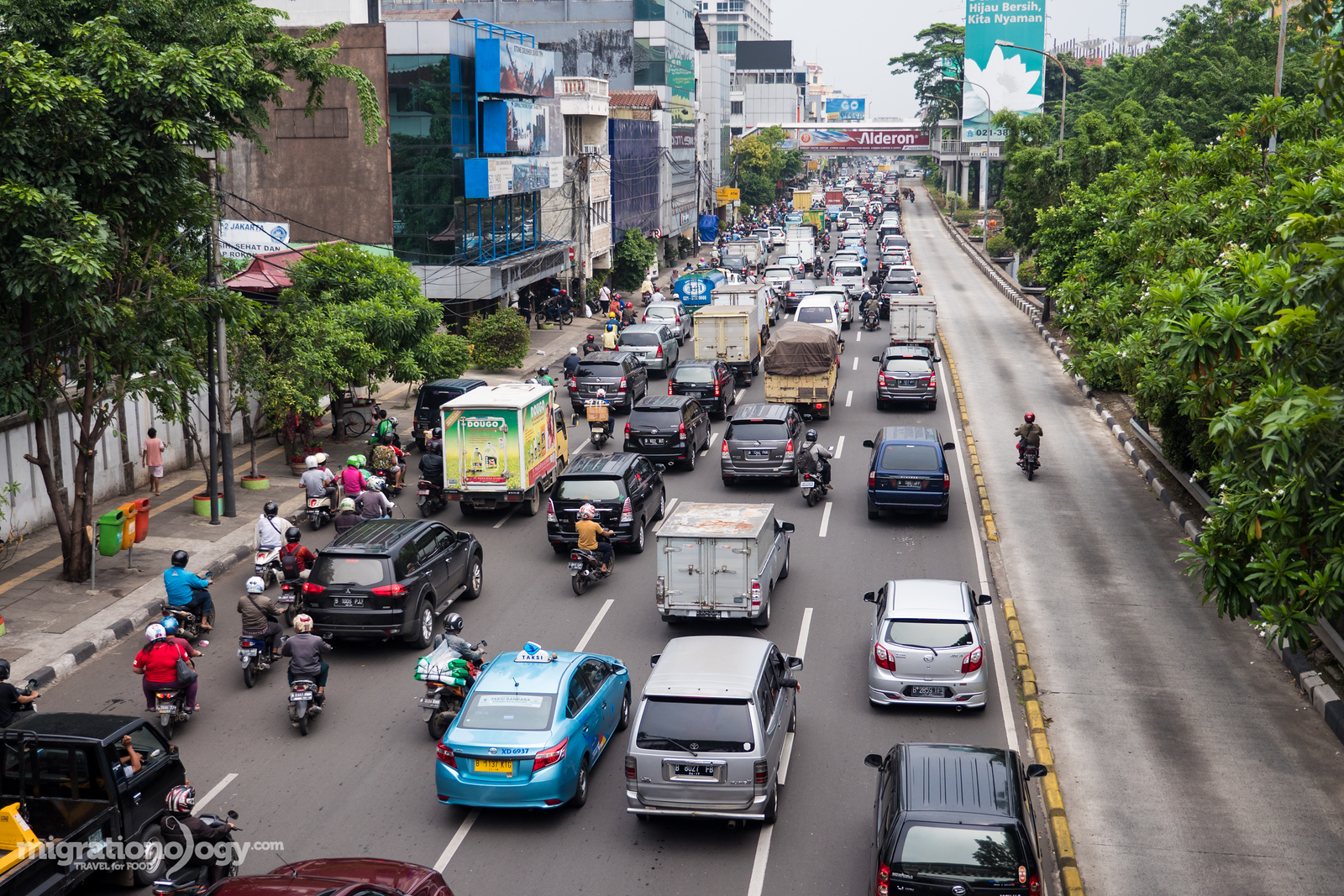
That’s not to say Jakarta is hassle free, it has its share of problems and crazy traffic, but if you’re up for it, Jakarta will reward you with some unforgettable meals and smiles.
Let’s get started…
Jakarta travel guide for food lovers
Arriving and leaving
If you’re flying into Jakarta on an international flight, you’ll probably arrived at Soekarno–Hatta International Airport, located in west Jakarta.
To get to the center of the city, it’s easiest to jump into a taxi – I would recommend Blue Bird company – and go directly to your hotel or wherever you’re staying. The fare by taxi should cost about 120,000 – 150,000 Rupiah from the airport to the center of Jakarta.
Once you exit baggage claim, find a line for Blue Bird, and there will be a little stand somewhere with an official who gives you a queue number for a taxi.
Our room at Veranda Hotel in Jakarta
Where to stay?
Jakarta is a massively spread out city, and so if you have something you need to do in a certain area, it’s a good idea to stay in that area. During my three week stay in Jakarta, I stayed in a couple of different areas of the city, to get a feel for more parts of the city.
In general, I would say the best area of Jakarta to stay in is as a traveler is central Jakarta, either just south of the National Monument (Kebon Sirih) or just north of the National Monument (Hayam Wuruk up to Mangga Besar).
Here are some hotels I would recommend:
Hotel Santika Premiere Hayam Wuruk – Newly built and very modern, Hotel Santika Premiere Hayam Wuruk is part of a local Indonesian hotel brand. My wife and I paid about $45 USD per night and we stayed for a week. It was quite a good value hotel, and the location, right on Hayam Wuruk and Mangga Besar is very good. Plenty of delicious food in the area.
Veranda Hotel – In order to experience a completely different side of Jakarta, in the heart of South Jakarta in an area called Gandaria, my wife and I checked into the Veranda Hotel. The hotel itself is new and very nice. The internet was blazing fast, and there a nice mall right around the corner. And on top of that, there’s a lot of excellent Indonesian food (less Chinese food) in the area. The only thing is, it’s a bit far from the center of Jakarta, but not too bad. Overall, an excellent place to stay.
*Affiliate links – If you make a booking, at NO extra expense to you, I will get a small commission. Thank you for your support.
Indonesian food – restaurants and street food
Restaurants and Street Food
Indonesia is a country that’s made up of over 17,000 islands. Not all of them are inhabited, but there are still many that are, and so the diversity of people, culture, and different foods is astounding. One of the best things about eating in Jakarta is that, being the largest and most influential capital city of Indonesia, people come from all different islands, and so you’ll be able to discover food from all over Indonesia somewhere in Jakarta.
Sometimes when I was eating at street food stalls and restaurants in the city, I hardly even knew what island or culture cuisine I was eating, until finishing my meal and doing some research – and that’s a wonderful thing, because there’s so many different styles of Indonesian food.
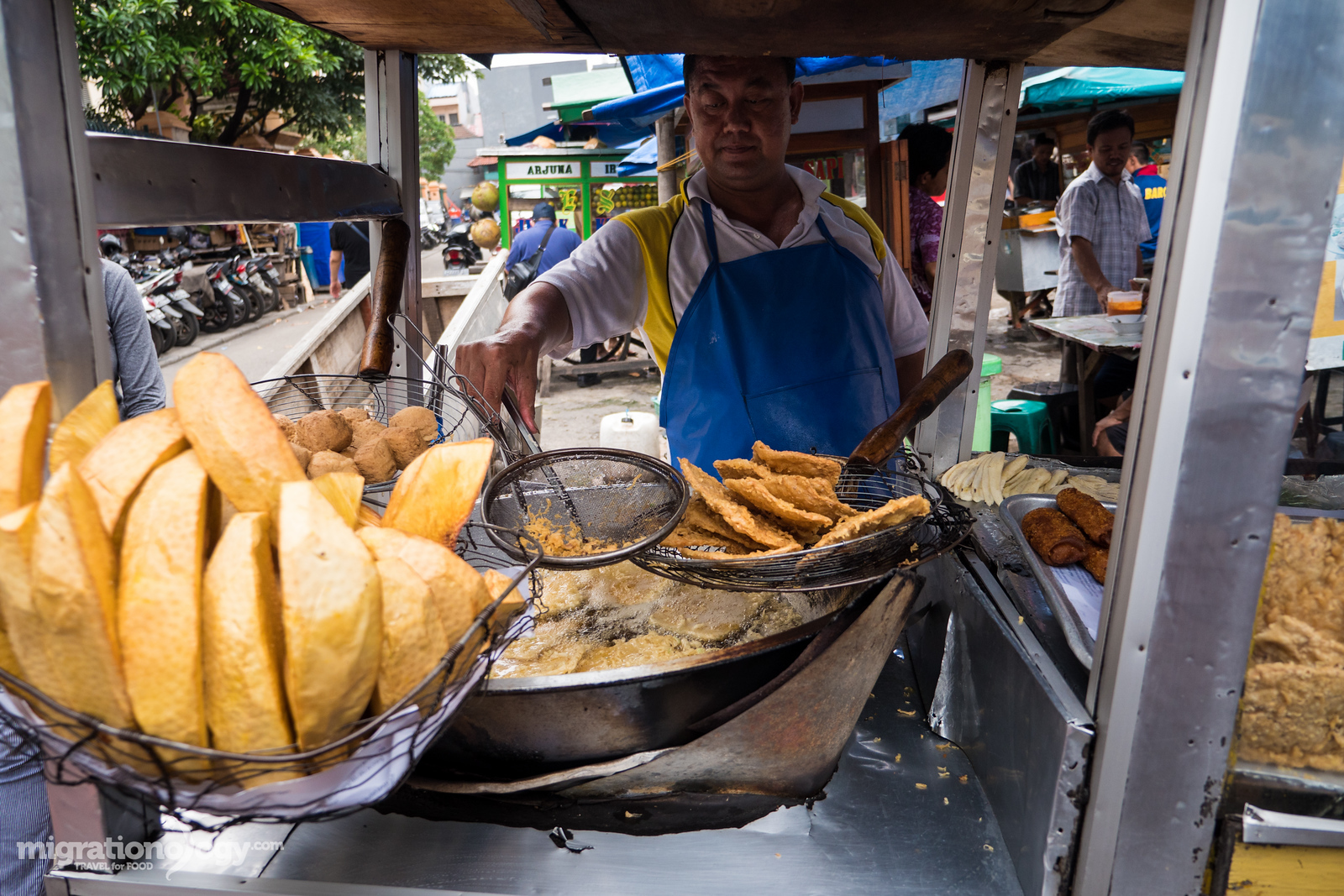
All sorts of deep friend snacks – deep fried breadfruit, one of my favorites.
There are two frequent types of street food available in Jakarta:
Warung – A warung typically refers to a small family run restaurant, often in a small shelter style building, but it’s typically a permanent place as opposed to a mobile street food cart.
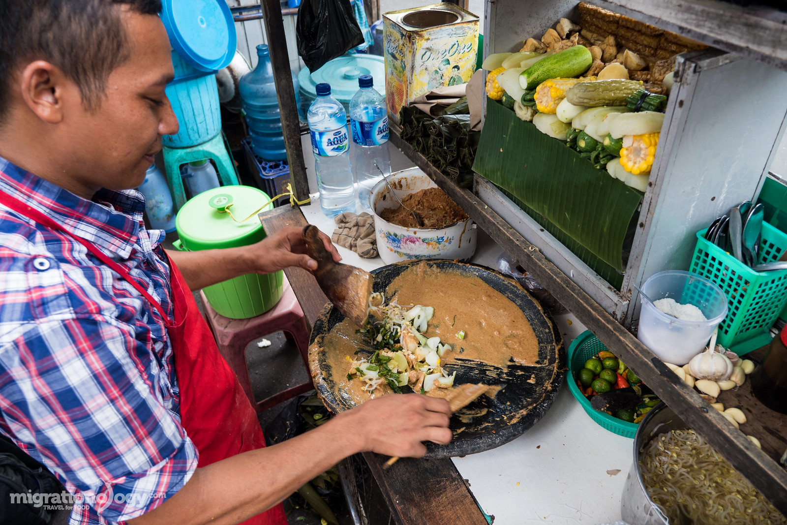
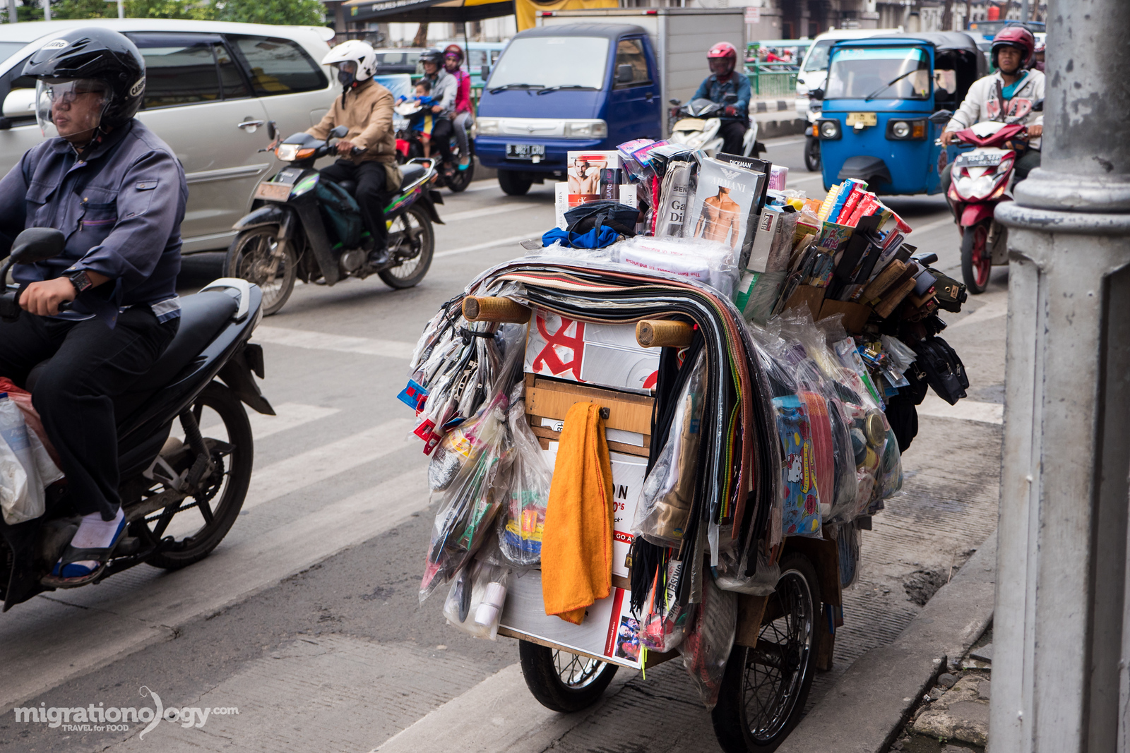
Pedagang kaki lima – Literally meaning a five feet trader, pedagang kaki lima is a term used to describe street food carts in Indonesia. Typical carts have two wheels, a leg stand, and then the two legs of the vendor, making five legs in total. You’ll find all sorts of amazing things to eat from street food vendors in Jakarta, ranging from curries and sate, to deep fried snacks and gado gado.
These are the two main styles of dining I focused on during my time in Jakarta, and along with having some seriously delicious food, I also found that many of the sellers, at both local warung’s and street food stalls were very friendly and kind.
Amazing Indonesian food!
A few of my favorite Indonesian dishes:
For a more complete list of Indonesian food in Jakarta, see my full guide (coming soon), but this is just a brief overview of a few of my personal favorites.
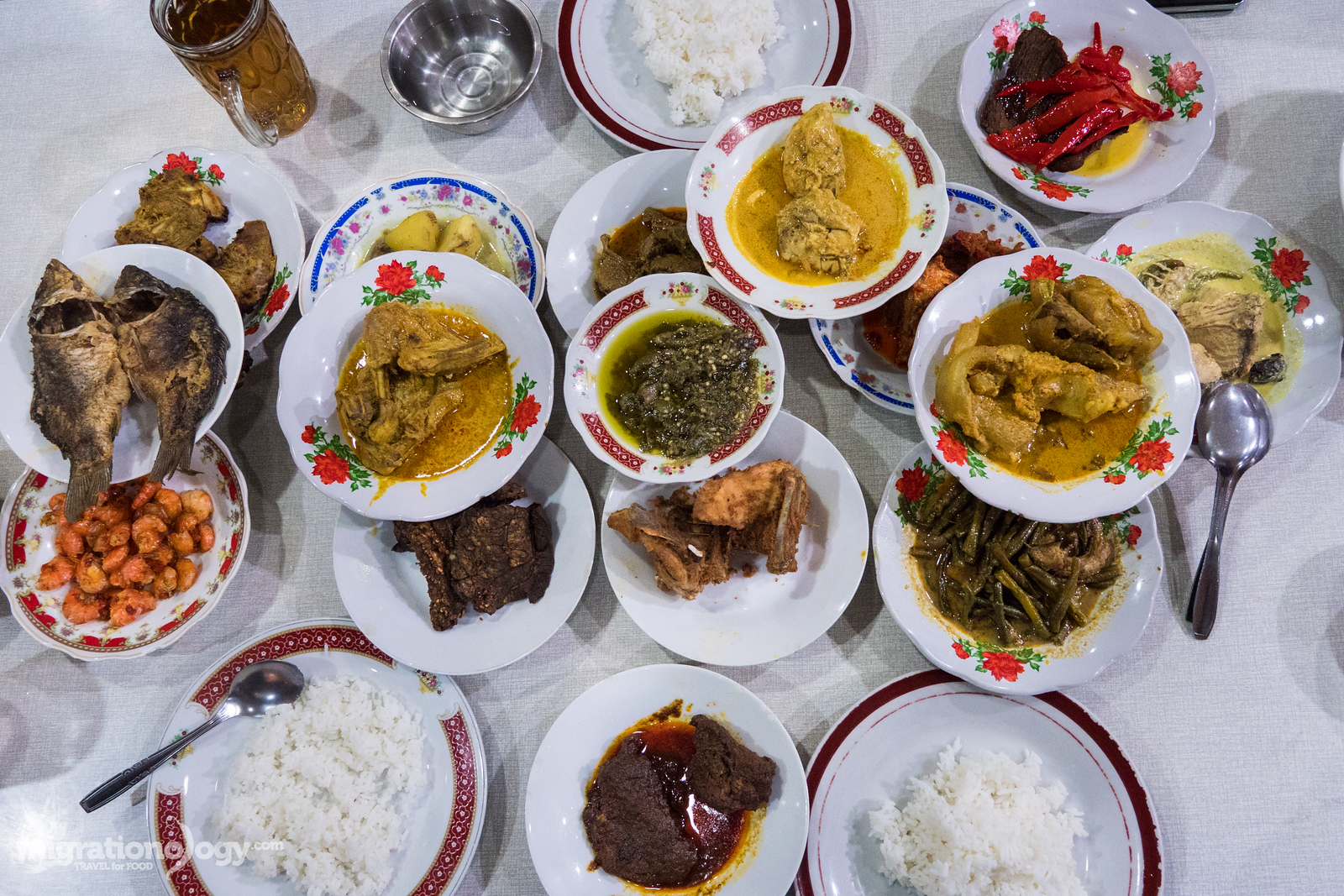
Nasi Padang – Ever since visiting the island of Sumatra back in 2010, I’ve been a little obsessed with food originating in Padang, a province on the west coast of Sumatra. When you eat Nasi Padang it’s a full meal of a variety of different curries, prepared with lots of fresh herbs and spices, coconut milk, and plenty of chilies. Nasi Padang is one of my favorite meals in the world.
Nasi uduk – Nasi uduk, rice cooked with coconut milk and a few fragrant spices, is commonly found throughout Jakarta. It can be served with a variety of different deep fried things, like deep fried chicken and tofu, with sambal chili sauce, or it can be served with a variety of different local curries and side dishes. The rice itself is so good and fragrant.
Soto Betawi – Soto is the word used to describe a soup, and nearly every region of Indonesia has their own version of soto. Soto Betawi is from the people native to Jakarta, so it’s true Jakartan food. The soup is typically a little creamy, made with beef, and eaten with rice, and achar pickles. It’s an absolutely must eat Indonesian food in Jakarta.
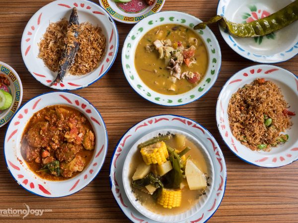
Woku – Woku is a dish from Manado, in the northern part of Sulawesi, that’s known for serving spicy and full flavor food. I liked just about every Manado dish I was able to try, but the woku, a blend of aromatic herbs and spices like turmeric, ginger, lemon basil, shallots, and tomatoes, all mixed and pounded together with fish (or something else), was one dish that I couldn’t get over. It’s an amazing dish to eat.
Sop kaki kambing – Known as goat leg or feet soup, but can include all sorts of random goat organs as well, sop kaki kambing is an Indonesian food dish that only for goat lovers. The dish is commonly served at warung’s, and you often choose any parts of the goat that you want, they will slice them up into a bowl, mix it with soup, and it’s eaten with rice and pickles.
Ikan bakar – I absolutely love the way fish is grilled in Indonesia. They often begin by butterfly cutting, so that there’s a maximum surface area for both the sambal marinade and the charcoal. Once the fish is slightly blacked from the high fire grilled process, it’s then served with fresh lime (or calamansi), and eaten with either sambal chili sauce, or kecap manis (sweet soy sauce) and diced chilies.
Gado gado – One of the most common Jakarta street food dishes is gado gado, a salad of vegetables and rice cakes (lontong), all coated in a thick and creamy peanut sauce. Gado gado can make a great light meal, or a snack, and you’ll especially find it being sold throughout Jakarta from mobile street food carts.
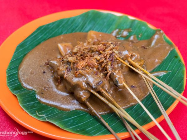
Sate Padang – Trying sate Padang, again from the Padang province of Sumatra in Indonesia, for the first time was a huge surprise. It just honestly didn’t look all that good. But I was in for a flavor explosion on my first skewer – the spice blend coated onto the meat just protruded with spices like cumin and turmeric, and the sauce just sort or melted around the meat. The crispy shallots on top added an extra touch. An amazing dish you’ve got to try, completely different from other variations of Indonesian sate.
Ayam bakar taliwang – Originating from the island of Lombok, ayam bakar is a type of grilled small baby chicken that’s known for being chili filled and spicy. They normally use country chickens, which are quite small, but very flavorful in a natural kind of tasting way, and have slightly chewy texture. The chicken are marinated and grilled with a choice of powerful chili sambal caked all over them. Eating ayam bakar Taliwang was a little bit of a life changing grilled chicken experience for me.
Sambal – I couldn’t make an Indonesian favorite food list without including sambal, any variety of different chili based sauce or garnish. You’ll be eating sambal with just about every meal you have in Indonesia, and no two are the same. There must be thousands of different sambal versions, even some families have their own unique one, and it provides extraordinary flavor to just everything.
These are just a few of the dishes and meals you can eat in Jakarta. There are many others as well, but this is a start of a few of my favorites.
Jakarta is a melting pot of Indonesian cuisine from around the country. But one of the regional cuisines that seems to be underrepresented is food from the Betawi people, who are the original inhabitants of the present day area of…
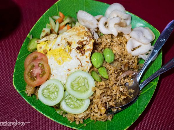
Nasi Goreng Petai (Stink Bean Fried Rice) at Mangga Besar
12 Comments
Nasi goreng, fried rice, is easily one of the most famous Indonesian foods. I wouldn’t call it one of the top Indonesian foods, but I do think everyone can enjoy a plate of nasi goreng from time to time, and I certainly…
Flavor Explosion at Sate Padang Ajo Ramon in Jakarta
9 Comments
Have you ever had a plate of food sitting on the table before you that doesn’t look very pretty? But then you take your first bite, and you’re blown away by how delicious it is? That’s exactly what happened to me…
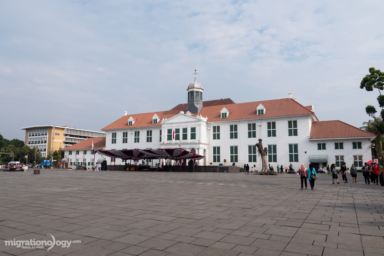
Fatahillah Square – Jakarta Old Town
Things to do in Jakarta
Being a food lover, and focusing mostly on eating when I travel, I’m not all that concerned about chasing famous attractions when I travel. But that being said, it is nice to occasionally (like in-between meals) to do some sightseeing.
I think part of the reason why Jakarta doesn’t always get too much light as a tourist destination is because there’s not really all that much to do and see in terms of famous buildings, museums, sights, or natural wonders (that is right in Jakarta).
However, there are a few things, and there’s also a big art scene and shopping culture as well.
National Museum of Indonesia – Located just to the west side of Merdeka Square is the National Museum. The museum houses a great collection of Archaeology and Ethnography collections from around Indonesia. If you enjoyed walking visiting museums, it’s a good place go when you’re in Jakarta.
Monas (National Monument) – Built as a symbol for the Indonesia struggle for freedom, the National Monument is located right in the center of Jakarta in Merdeka Square. The monument is located in the middle of a huge park, and you can go to the top of the monument for a fee of 5,000 IDR for a pretty good view of the city.
Istiqlal Mosque and Jakarta Cathedral – Not only the largest mosque in Indonesia, but also in Southeast Asia, Istiqlal Mosque can host 120,000 people at a time. After removing your shoes, you can walk around and get a tour of the mosque. Right across the street, and another icon of Jakarta is the Jakarta Cathedral, a large Roman Catholic Cathedral built in 1901.
Jakarta Old Town – Also known and Old Batavia or Kota Toa, this area of northern central Jakarta is where you’ll find many of the old colonial Dutch buildings. Fatahillah Square is a good place to start, and there are a number of museums in the area, and you can even rent a pink bicycle and ride around if you’re up for it.
Glodok (Chinatown) – Along with eating, I like to explore markets and food areas of cities when I travel. Glodok, which is the Jakarta name for their Chinatown, is a very interesting around of the city to walk around, explore, and eat through. There are a few lanes within the center of Glodok where you can walk around local markets and stop at food stalls. I also really enjoyed a cup of coffee at the legendary Kopi Es Tak Kie.
Additionally, you’ll find dozens of modern malls scattered throughout Jakarta, and it seems that walking around air-conditioned malls on the weekends is a pretty popular thing to do.
But of course, I say the best thing to do in Jakarta is eat, and there’s no shortage of food to try, no matter how long you stay in Jakarta.
Jakarta reminds me in a lot of ways of Bangkok, but Bangkok with its BTS and MRT, make it a little easier to avoid traffic using public transportation. Jakarta on the other hand, for as big and populated a city as it is, transportation is not quite as convenient as it could be. Although I’ve heard a rail type of MRT or elevated train is in the thoughts, no one really knows if something like that will happen in the near future.
Taxi – One of the most reputable taxi companies in Jakarta, and throughout Indonesia, is Blue Bird. They have a booking app, or you can just wave one down on the street. Prices are affordable at about 20,000 – 50,000 Rupiah for a short ride and 100,000 – 150,000 for a long ride.
UberX (<- If you use this link, we’ll both get a FREE ride) – For almost my entire travel trip in Jakarta my wife and I used UberX. We had great experiences with good drivers, and the vehicles are usually Toyota Avanza mini-vans, or equivalents. Sometimes we had to wait about 15 minutes for our UberX to arrive, but usually just about 5 minutes in Central Jakarta. Prices are typically a little cheaper than traditional taxis. For a short ride you’ll pay about 20,000 – 40,000 Rupiah and for a ride across town it might cost 80,000 – 120,000 Rupiah. If you sign up with this link, we’ll each get a free ride.
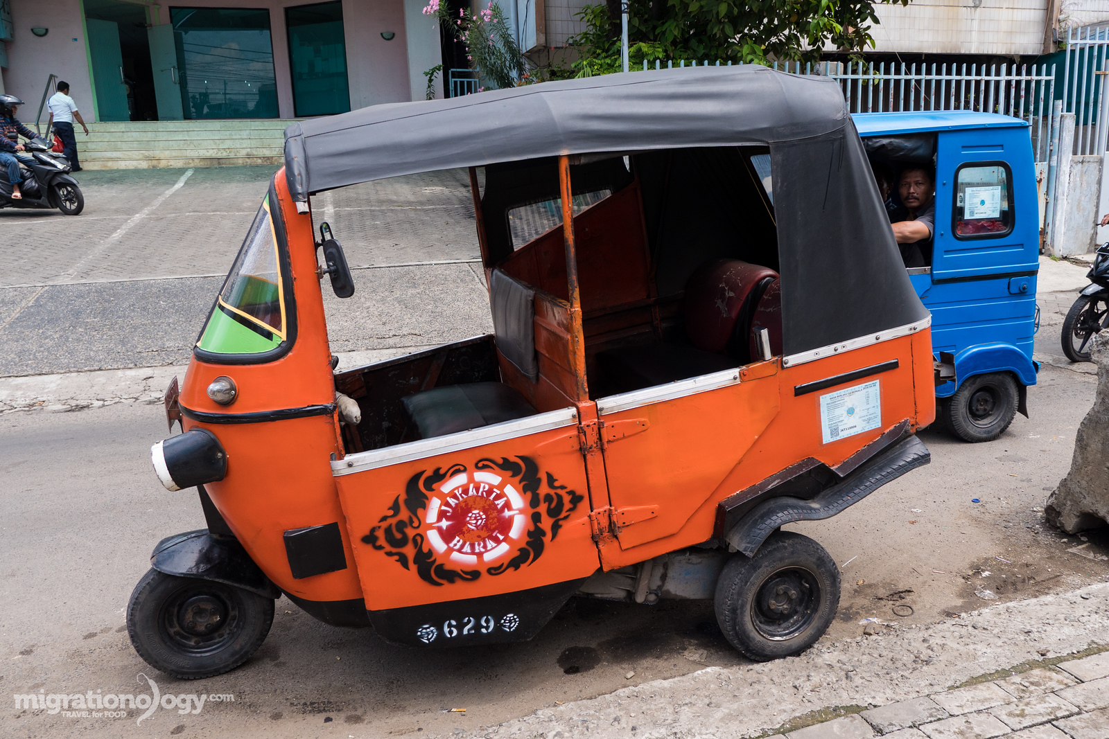
Bajaj – Also known as an auto-rickshaw, a bajaj are the mini three-wheelers, that just like in India, prowls the streets, and offer convenient short distance transportation. I particularly like the old orange rickshaws, but there are also newer looking blue rickshaws from India.
Motorbikes (known as Ojek ) – Motorbikes are a very common (and quick) way to get around Jakarta, and they are frequently used as motorbike taxis.
Go Jek – Go Jek is an app for booking a motorbike to take you anywhere or do other things for you (like order street food to deliver to you). It’s very convenient, and it charges a set fee, so you don’t have to worry about getting ripped off, and they provide you with a helmet. Good information on this blog post.
There are also buses, and the TransJakarta bus system, but I honestly stuck mostly to using UberX and Bajaj rickshaws during my visit to Jakarta.
Traffic is one of the biggest hardships or hassles of living in or traveling to Jakarta. There’s no real way around the notorious traffic jams. However, I found that if you can avoid the peak rush hours (when traffic is the worst), it’s not too bad. Just give yourself time getting places, don’t be in a rush to get somewhere as fast as possible, and you’ll be fine.
Prices and expenses in Jakarta
Prices and Expenses
Accommodation:
Hostel – $10 – $25 USD per bed
Mid-range hotel – $25 – $60 USD per night
High end – Everything above $60 USD
Transportation:
Taxi ride – For short rides you’ll probably spend 20,000 – 50,000 Rupiah and for longer rides across town you’ll spend about 100,000 – 150,000 Rupiah
UberX ride (If you use this link, you and I will both get a free ride) – UberX is very affordable in Jakarta. For short rides you’ll spend about 20,000 – 40,000 Rupiah, for treks across town you might spend 100,000 – 150,000 Rupiah.
Bajaj ride – It’s hard to tell, very much depending on distance and traffic, but a short ride might cost 10,000 – 20,000 Rupiah
Motorbike ride (ojek) – 10,000 – 40,000 Rupiah
Food:
Street food single dish – 10,000 – 20,000 Rupiah
Local restaurant – 20,000 – 60,000 Rupiah per person
Indoor restaurant – 100,000 – 300,000 Rupiah per person or more
When I was in Jakarta, my wife and I made food videos of many of the restaurants and street foods that we ate during our visit. You can watch the videos below:
Jakarta is not the most talked about city to visit as a tourist in Southeast Asia. But if you choose to visit, with an intent to try lots of delicious food, I think it’s a city that offers so many rewards.
One of the things I love about Indonesia is how diverse it is, consisting of thousands of islands, and Jakarta is the melting pot, the collision of all cultures and foods from around the country.
When you’re in Jakarta get ready to experience the vibrant culture and food of Indonesia!
Have you been to Jakarta? Or to another part of Indonesia?
I would love to hear from you in the comments section below about your favorite Indonesia food…
If my guide and videos were helpful, please consider making a donation or purchasing something from the store. With your help, I’ll be able to continue publishing Ad-Free travel guides. Thank you in advance!
Enter your email & I'll send you the best food updates